Chapter 2 — Design Methods
This chapter presents the executable design principles, failure mechanism mapping, and decision logic that guide the engineering of surface water monitoring systems. It provides structured frameworks for translating site conditions and monitoring objectives into specific component selections, QA/QC strategies, and lifecycle cost considerations.
2.1 Executable Design Principles and Basis
Sound system design for surface water monitoring is grounded in a set of engineering principles derived from field experience, metrology practice, and regulatory requirements. These principles are not aspirational guidelines but executable criteria that must be verified during design review and acceptance testing. The table below presents twelve core principles with their rationale, applicability conditions, and basis type.
| Principle | Why It Matters | Applicable When | Basis Type |
|---|---|---|---|
| Representative intake placement | Avoid biased samples from surface algae or bottom sediment | All sites | Hydrology practice + field survey |
| Anti-fouling first, accuracy second | Unattended stability dominates long-term data quality | Remote/unmanned stations | O&M reality + lifecycle cost analysis |
| Measure flow or stage with context | Interpret concentration changes in hydrological context | Rivers and reservoir outflows | Hydrologic analysis practice |
| Always implement validity flags | Trust requires traceability to instrument status | Regulatory reporting applications | Audit requirement |
| Design for clogging and sediment | Biggest single cause of system downtime | High turbidity / seasonal flood sites | Field failure statistics |
| Edge buffering ≥ worst expected outage | Prevent permanent data gaps during network failures | Cellular network deployments | Telecom reliability data |
| Calibration workflows are part of the system | All sensors drift; calibration must be scheduled and logged | All deployments | Metrology practice |
| Lightning/grounding as core, not optional | Outdoor sites are exposed; surge damage is catastrophic | Storm-prone regions | Electrical safety standards |
| Secure remote access by design | Unmanned stations increase cyber attack surface | All deployments | Cybersecurity standard practice |
| Modular replacement strategy | Field swaps reduce mean time to repair (MTTR) | Multi-site networks | Maintainability engineering |
| Separate measurement and lab sampling | Different integrity chains; cannot substitute one for the other | Drinking water source protection | QA/QC methodology |
| Hydrology + meteorology time alignment | Event analytics depends on correct temporal context | All deployments | Time-series analytics practice |
2.2 Failure Causes and Engineering Avoidance
A systematic understanding of failure mechanisms is essential for designing systems that achieve the target uptime and valid data ratio. The following table maps ten common failure causes to their underlying mechanisms and the engineering measures that prevent or mitigate them. Each measure has been validated through field deployments across diverse river and lake environments.
| Failure Cause | Mechanism | Engineering Avoidance |
|---|---|---|
| Intake clogged by debris | Leaves, plastics, and fibrous material block strainer | Dual strainer + automatic backflush + debris guard + seasonal maintenance schedule |
| Bubble intrusion | Pump cavitation, poor venting, or turbulent intake | Bubble trap + degasser + correct suction head + flow cell venting |
| Biofouling on optics | Algae films form on optical windows in warm, nutrient-rich water | Wipers + copper anti-fouling rings + anti-fouling coatings + adaptive cleaning schedule |
| Sensor drift | Membrane aging, reagent degradation, or reference electrode depletion | Calibration plan + consumable tracking + spare sensor kits on site |
| Condensation in cabinet | Temperature swings cause moisture to condense on electronics | Cabinet heater/ventilation + desiccant + IP-rated cable glands |
| Lightning surge | Induced voltage on exposed cables and antenna feeds | SPD on AC and signal lines + single-point grounding + fiber isolation where feasible |
| Cellular instability | Tower congestion, weak signal, or SIM expiry | Local buffer + store-and-forward + dual SIM + adaptive reporting interval |
| Vandalism/theft | Remote sites targeted for equipment or cable theft | Tamper switch + optional CCTV + hidden conduits + robust locks + asset tags |
| Mud/silt in floods | Submergence of cabinet or intake during high water events | Elevated mounting + flood-rated enclosure + quick-disconnect fittings |
| Misleading alarms | Alarms triggered without hydrological or sensor-health context | Multi-sensor correlation + alarm suppression under invalid sensor states |
2.3 Core Design and Selection Logic
The design selection process follows a structured decision path that begins with water body characterization and ends with a validated bill of materials and acceptance criteria. The decision tree below illustrates the key branching points, from water body type through hydrodynamics, turbidity regime, access conditions, and power availability, to the recommended station type. This visual framework helps designers rapidly identify the appropriate configuration and avoid over- or under-specifying the system.
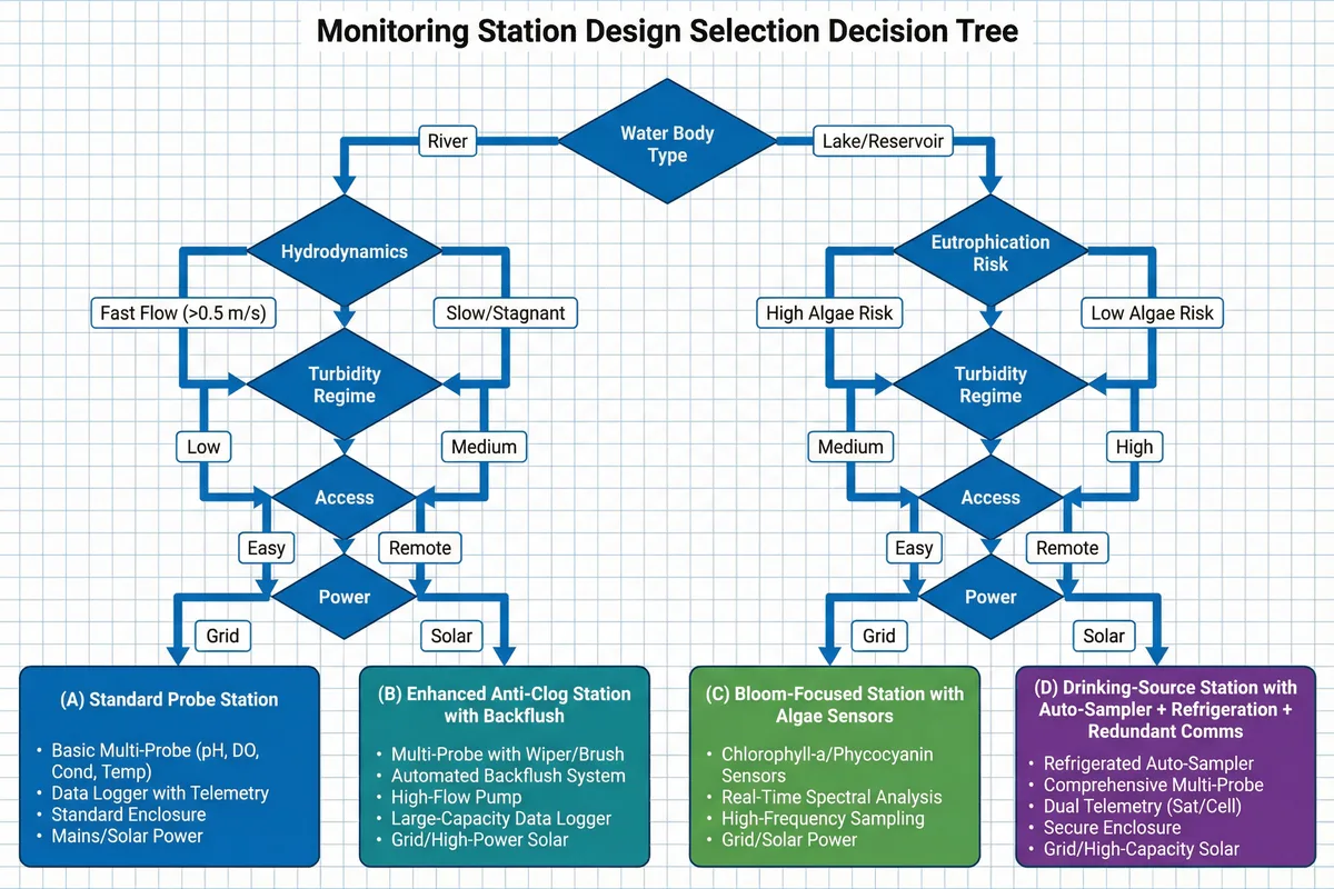
Figure 2.1: Design selection decision tree — from water body type to recommended station configuration
The complete design decision sequence is as follows:
- Define monitoring objectives (regulatory compliance, trend analysis, event detection, source tracing)
- Define target parameters and accuracy bands for each parameter
- Conduct site survey: flow velocity, depth profile, debris regime, seasonal patterns, access, security
- Select intake type and pre-treatment configuration based on turbidity and debris load
- Select sensors and analyzers based on parameter requirements and fouling risk
- Size power system (grid, solar, battery, UPS) based on load and autonomy requirement
- Design communications (primary 4G/5G, backup NB-IoT/LoRa, satellite for extreme remote)
- Define QA/QC rules and validity flag taxonomy
- Define integration requirements and reporting formats
- Run lifecycle cost check (CapEx + OpEx over 5–10 years)
- Finalize BOM and acceptance criteria
2.4 Key Design Dimensions
Beyond the component selection logic, system design must address six key dimensions that collectively determine the long-term performance and cost-effectiveness of the monitoring network. These dimensions are interdependent and must be balanced against site-specific constraints and budget realities.
| Dimension | Key Considerations | Design Targets |
|---|---|---|
| Performance / Experience | Alarm latency, dashboard responsiveness, field usability | Alarm delivery ≤ 5 min; dashboard load ≤ 3 s; field UI operable with gloves |
| Stability / Reliability | Uptime, MTBF, power autonomy, anti-fouling effectiveness | Valid data ratio ≥ 85–95%; autonomy ≥ 3–7 days; cleaning interval ≥ 7 days |
| Maintainability | Modular swaps, tool-less access, consumable logistics | Probe replacement ≤ 30 min; filter replacement ≤ 15 min; no special tools required |
| Compatibility / Expandability | Open protocols, spare IO ports, platform APIs | Modbus RTU/TCP; JSON payloads; versioned schemas; ≥ 2 spare sensor ports |
| Lifecycle Cost (LCC) | Reagents, site visits, failure-driven replacements | OpEx ≤ 20–30% of CapEx per year for well-designed systems |
| Energy & Environment | Solar sizing, low-power modes, reagent waste handling | Solar autonomy ≥ 5 days at remote sites; waste reagent containment provided |